inv_links <- list(
  identity = function(eta) eta,
  inverse = function(eta) 1/eta,
  log = exp)

get_data <- function(inv_link){
  x <- pmin(pmax(0, rnorm(n, 2)), 4)
  z <- pmin(pmax(0, rnorm(n, 1)), 4)
  eta <- 1 + x + 2*z
  data.frame(
    x=x,
    z=z,
    eta=eta,
    mu=inv_link(eta),
    y=rgamma(n, shape=1, scale=inv_link(eta))
  )
}

is.in.confint <- function(x, I) (x >I[1]) && (x< I[2])Simulate a glm with exponential distribution such that
\[\operatorname{y} \sim \operatorname{exp}(\operatorname{h}(\alpha + 1\operatorname{x} + 2\operatorname{z}))\]
with the \(h\) being the inverse of the link functions:
- identity
- inverse
- log
Setup
Simulation
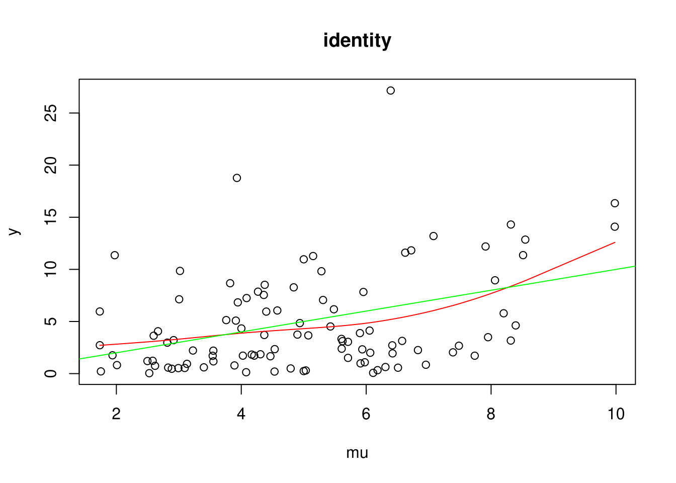
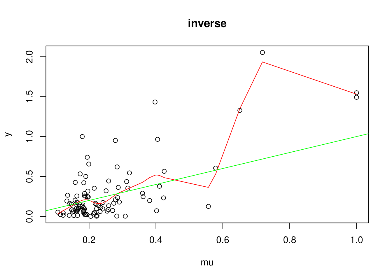
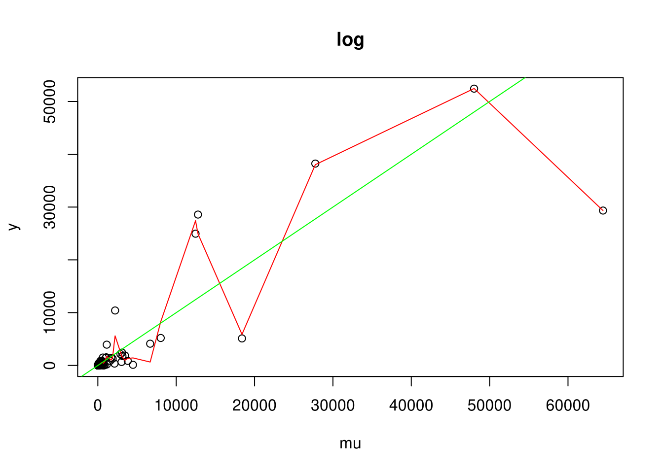
For each link function: 1. Plot an example (green line is the true expectation and red line is a smoothing spline) 2. Simulate coverage of true parameter for x (should be 95%)
n <- 100 # sample size
nsim <- 500 # number of simulations to test the confidence interval
set.seed(123)
for (i in seq_along(inv_links)){
  D <- get_data(inv_links[[i]])

  plot(y ~ mu, main=names(inv_links)[i], data=D)
  # Test with SmoothingSplines if indeed: E(y|mu) = mu
  with(D, lines(smooth.spline(mu, y), col='red'))
  abline(0,1, col='green')

  # see if the conf-interval for beta_x is valid. i.e.:
  #    repeat it nsim times and see if 1 is in our confidence interval
  R <- mcreplicate::mc_replicate(nsim,{
    try({
      D <- get_data(inv_links[[i]])
      s <- summary(f <- glm(
        y ~ x + z,
        data = D,
        family = Gamma(link = names(inv_links)[i]),
        mustart = mu)); s
      suppressMessages(is.in.confint(1, confint(f, "x")))
    }, silent = TRUE)
  })
  coverage <- mean(as.logical(R), na.rm=TRUE)
  cat(sprintf("Coverage for %s: %f\n", names(inv_links)[i], coverage))
}
Coverage for identity: 0.940299
Coverage for inverse: 0.946058
Coverage for log: 0.956000Results
For all link functions, the coverage is about 95%