Setup + Preprocessing
suppressPackageStartupMessages ({library (dplyr)library (ggplot2)library (egg)library (kernlab)library (mgcv) # for GAM models - smoothing library (gridExtra) # for combining plots library (tidyr) # for pivoting data theme_set (theme_minimal ())options (digits = 3 )source ("R/data_prep.R" )
Number of matches per filter criteria (not disjoint)
  Headphone  PRS_all_NA    Distance Activity_NA    Duration  HMNoise_NA
        303         226         221         102          96          96
JourneyTime
         20
Keep  1494 of 2206 observations
Code
$ RL_NDVI <- pmax (0 , D$ RL_NDVI)$ RL_NDVI <- pmax (0 , D_trn$ RL_NDVI)$ RL_NDVI <- pmax (0 , D_tst$ RL_NDVI)$ LANG <- as.factor (D$ LANG)$ LANG <- as.factor (D_trn$ LANG)$ LANG <- as.factor (D_tst$ LANG)$ SEX <- as.factor (D$ SEX)$ SEX <- as.factor (D_trn$ SEX)$ SEX <- as.factor (D_tst$ SEX)$ JNYTIME <- D$ JNYTIME + quantile (D$ JNYTIME[D$ JNYTIME > 0 ], 0.05 , na.rm= TRUE )/ 2 $ JNYTIME <- D_trn$ JNYTIME + quantile (D_trn$ JNYTIME[D_trn$ JNYTIME > 0 ], 0.05 , na.rm= TRUE )/ 2 $ JNYTIME <- D_tst$ JNYTIME + quantile (D_tst$ JNYTIME[D_tst$ JNYTIME > 0 ], 0.05 , na.rm= TRUE )/ 2 $ DISTKM <- D$ DISTKM + quantile (D$ DISTKM[D$ DISTKM > 0 ], 0.05 , na.rm= TRUE )/ 2 $ DISTKM <- D_trn$ DISTKM + quantile (D_trn$ DISTKM[D_trn$ DISTKM > 0 ], 0.05 , na.rm= TRUE )/ 2 $ DISTKM <- D_tst$ DISTKM + quantile (D_tst$ DISTKM[D_tst$ DISTKM > 0 ], 0.05 , na.rm= TRUE )/ 2 $ SPEED_log <- log (D$ DISTKM / D$ JNYTIME)$ SPEED_log <- log (D_trn$ DISTKM / D_trn$ JNYTIME)$ SPEED_log <- log (D_tst$ DISTKM / D_tst$ JNYTIME)# logical_vars <- c("ALONE","WITH_DOG","WITH_KID","WITH_PAR","WITH_PNT","WITH_FND") # D[logical_vars] <- lapply(D[logical_vars], as.numeric) # D_trn[logical_vars] <- lapply(D_trn[logical_vars], as.numeric) # D_tst[logical_vars] <- lapply(D_tst[logical_vars], as.numeric)
Train/test split
<- names (D)grep ("HM|RL" , nams)]
 [1] "HM_NOISELVL" "HM_NDVI"     "HM_NOISE"    "RL_NDVI"     "RL_NOISE"
 [6] "HM_COORDX"   "HM_COORDY"   "RL_COORDX"   "RL_COORDY"   "RL_GCOORD"
[11] "RL_GCOORDN"  "RL_GCOORDW"
Train/test split
<- c (# "HM_NOISELVL", # "HM_COORDX","HM_COORDY","RL_COORDX","RL_COORDY","RL_GCOORD", # "RL_GCOORDN","RL_GCOORDW", "HM_NDVI" ,"HM_NOISE" ,"RL_NDVI" ,"RL_NOISE" ,"ALONE" ,"WITH_DOG" ,"WITH_KID" ,"WITH_PAR" ,"WITH_PNT" ,"WITH_FND" ,"LANG" , # "AGE","SEX", "DISTKM_sqrt" , "JNYTIME_sqrt" , "SPEED_log" <- D_trn[vars]<- D_tst[vars]<- D_trn[complete.cases (D_trn), ]<- D_tst[complete.cases (D_tst), ]<- lapply (D_trn[], \(x) if (is.numeric (x)) scale (x) else x)<- lapply (D_tst[], \(x) if (is.numeric (x)) scale (x) else x)# summary(D[vars])
cor (cbind (D_trn[c ("DISTKM_sqrt" , "JNYTIME_sqrt" , "SPEED_log" )]))
             DISTKM_sqrt JNYTIME_sqrt SPEED_log
DISTKM_sqrt        1.000        0.473     0.713
JNYTIME_sqrt       0.473        1.000    -0.101
SPEED_log          0.713       -0.101     1.000
Remove DIST_sqrt, as it is highly correlated with the other two.
RL_NDVI
<- lm (RL_NDVI ~ (HM_NDVI + HM_NOISE + # ALONE + WITH_DOG + WITH_KID + WITH_PAR + WITH_PNT + WITH_FND + + # AGE + SEX + + JNYTIME_sqrt)^ 2 , D_trn)<- step (lm_ndvi, trace = FALSE , k = log (nrow (D_trn)))summary (fit <- lm (formula (step_ndvi), D_tst))
Call:
lm(formula = formula(step_ndvi), data = D_tst)

Residuals:
   Min     1Q Median     3Q    Max
-3.347 -0.426  0.178  0.682  1.874

Coefficients:
                       Estimate Std. Error t value Pr(>|t|)
(Intercept)             -0.2041     0.0859   -2.37   0.0179 *
HM_NDVI                  0.1572     0.0386    4.07  5.4e-05 ***
LANGGerman               0.2689     0.0972    2.77   0.0058 **
LANGItalian             -0.0768     0.1825   -0.42   0.6740
SPEED_log               -0.1112     0.0416   -2.67   0.0077 **
JNYTIME_sqrt             0.1059     0.0406    2.61   0.0094 **
HM_NDVI:SPEED_log       -0.1619     0.0399   -4.05  5.7e-05 ***
HM_NDVI:JNYTIME_sqrt    -0.1194     0.0395   -3.02   0.0026 **
SPEED_log:JNYTIME_sqrt  -0.0854     0.0394   -2.16   0.0308 *
---
Signif. codes:  0 '***' 0.001 '**' 0.01 '*' 0.05 '.' 0.1 ' ' 1

Residual standard error: 0.951 on 601 degrees of freedom
Multiple R-squared:  0.108, Adjusted R-squared:  0.0963
F-statistic: 9.11 on 8 and 601 DF,  p-value: 7.29e-12
R² = 0.08
Higher HM_NDVI corresponds to slightly higher RL-NDVI
higher JNYTIME_sqrt corresponds to slightly higher RL-NDVI
The faster (or further) you travel to RL, the more the RL_NDVI differs from HM_NDVI (negative interaction effect)
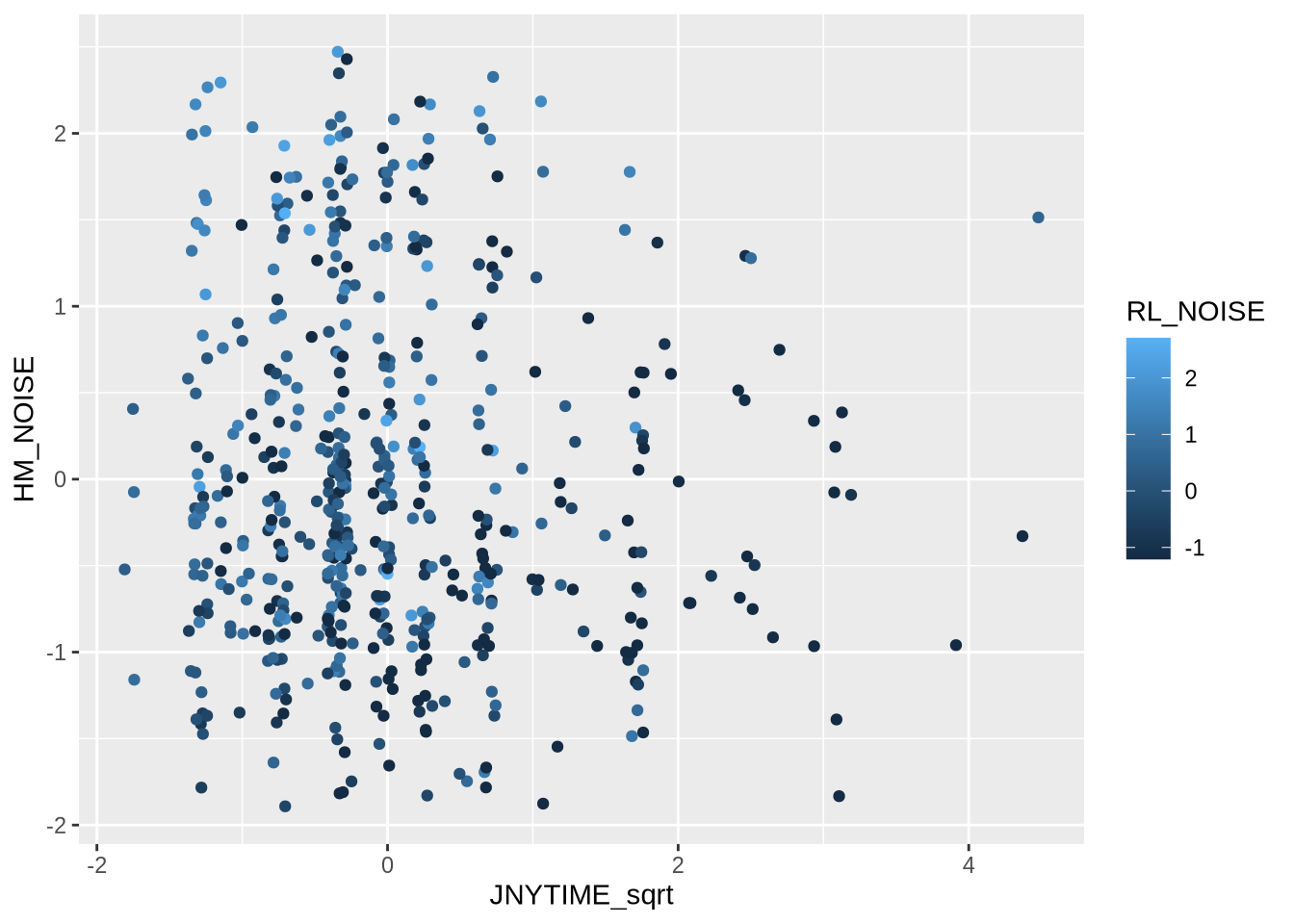
ggplot (D_tst, aes (x = JNYTIME_sqrt, y= HM_NOISE, col = RL_NOISE)) + geom_jitter (width= 0.07 , height = 0.1 )
RL_NOISE
<- lm (RL_NOISE ~ (HM_NDVI + HM_NOISE + # ALONE + WITH_DOG + WITH_KID + WITH_PAR + WITH_PNT + WITH_FND + + # AGE + SEX + + JNYTIME_sqrt)^ 2 , D_trn)<- step (lm_noise, trace = FALSE , k = log (nrow (D_trn)))summary (lm (formula (step_noise), D_tst))
Call:
lm(formula = formula(step_noise), data = D_tst)

Residuals:
    Min      1Q  Median      3Q     Max
-1.9524 -0.7719 -0.0133  0.6588  2.8255

Coefficients:
                       Estimate Std. Error t value Pr(>|t|)
(Intercept)           -0.000822   0.037211   -0.02    0.982
HM_NOISE               0.240824   0.037282    6.46  2.2e-10 ***
SPEED_log             -0.065753   0.037374   -1.76    0.079 .
JNYTIME_sqrt          -0.314663   0.037380   -8.42  2.8e-16 ***
HM_NOISE:JNYTIME_sqrt -0.037327   0.036309   -1.03    0.304
---
Signif. codes:  0 '***' 0.001 '**' 0.01 '*' 0.05 '.' 0.1 ' ' 1

Residual standard error: 0.919 on 605 degrees of freedom
Multiple R-squared:  0.161, Adjusted R-squared:  0.156
F-statistic: 29.1 on 4 and 605 DF,  p-value: <2e-16
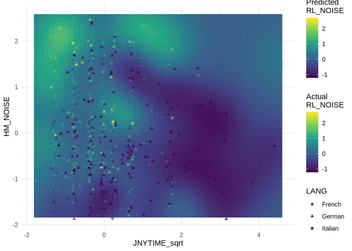
R² = 0.184
Participants can’t completely escape HM_NOISE (HM_NOISE positive predictor)
LANGItalians have it louder (than LANG de/fr)
Longer JNYTIME_sqrt leads to lower NOISE
Fit Gaussian Process for smooth plot
# Fit Gaussian Process <- as.matrix (D_tst[, c ("JNYTIME_sqrt" , "HM_NOISE" )])<- D_tst$ RL_NOISE# Fit GP with RBF kernel <- gausspr (X, y, kernel = "rbfdot" , kpar = "automatic" )
Using automatic sigma estimation (sigest) for RBF or laplace kernel
Fit Gaussian Process for smooth plot
# Create prediction grid <- range (D_tst$ JNYTIME_sqrt)<- range (D_tst$ HM_NOISE)<- expand.grid (JNYTIME_sqrt = seq (x_range[1 ], x_range[2 ], length.out = 50 ),HM_NOISE = seq (y_range[1 ], y_range[2 ], length.out = 50 )# Predict on grid $ predicted_RL_NOISE <- predict (gp_model, as.matrix (grid[, 1 : 2 ]))# Get combined range for both scales <- range (c (D_tst$ RL_NOISE, grid$ predicted_RL_NOISE))
Plot predicted RL_NOISE with GP
# Plot with matching color scales ggplot () + geom_raster (data = grid, aes (x = JNYTIME_sqrt, y = HM_NOISE, fill = predicted_RL_NOISE)) + geom_jitter (data = D_tst, aes (x = JNYTIME_sqrt, y = HM_NOISE, col = RL_NOISE, shape = LANG), width = 0.07 , height = 0.1 , alpha = 0.7 ) + scale_fill_viridis_c (name = "Predicted \n RL_NOISE" , limits = combined_range) + scale_color_viridis_c (name = "Actual \n RL_NOISE" , limits = combined_range)
$ PRS <- rowMeans (cbind (D$ FA,D$ BA,D$ EC,D$ ES))<- function (x) c (mean = mean (x, na.rm = TRUE ), sd = sd (x, na.rm = TRUE ), median = median (x, na.rm = TRUE ))aggregate (PRS~ HM_NOISELVL, D, summary_fun)
  HM_NOISELVL PRS.mean PRS.sd PRS.median
1           1    4.987  0.885      5.000
2           2    4.932  0.913      4.917
3           3    4.862  0.924      4.792
aggregate (FA ~ HM_NOISELVL, D, summary_fun)
  HM_NOISELVL FA.mean FA.sd FA.median
1           1    5.25  1.10      5.33
2           2    5.16  1.21      5.21
3           3    5.18  1.13      5.33
aggregate (BA ~ HM_NOISELVL, D, summary_fun)
  HM_NOISELVL BA.mean BA.sd BA.median
1           1    5.11  1.20      5.00
2           2    5.04  1.17      5.00
3           3    4.95  1.20      5.00
aggregate (EC ~ HM_NOISELVL, D, summary_fun)
  HM_NOISELVL EC.mean EC.sd EC.median
1           1    4.52  1.31      4.33
2           2    4.48  1.33      4.33
3           3    4.47  1.29      4.33
aggregate (ES ~ HM_NOISELVL, D, summary_fun)
  HM_NOISELVL ES.mean ES.sd ES.median
1           1    5.07  1.41      5.23
2           2    5.05  1.38      5.00
3           3    4.85  1.55      5.00